https://medium.com/@kaanerdenn/convolutional-neural-network-cnn-computer-vision-75f17400b261
Convolutional Neural Network (CNN) & Computer Vision
In this exploration of Convolutional Neural Networks (CNNs) and their pivotal role in the field of computer vision, we aim to lay the…
medium.com
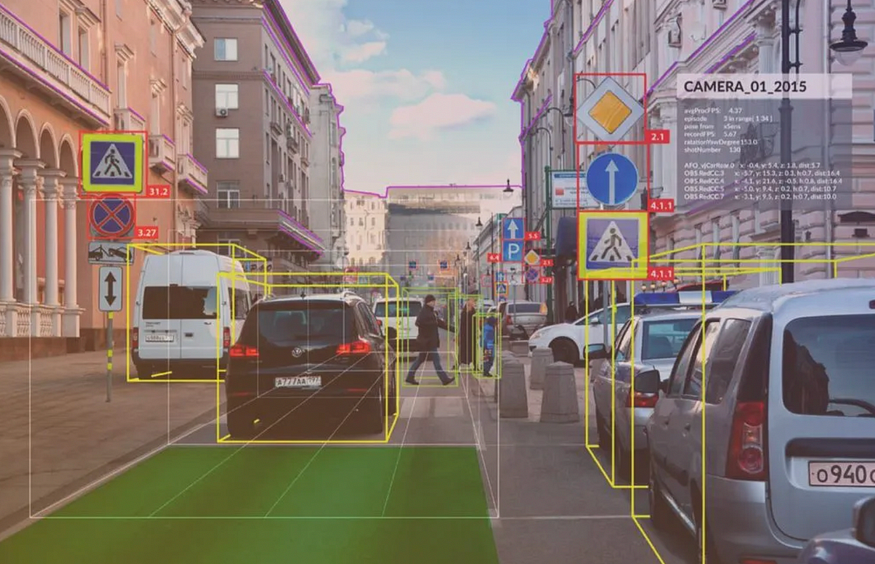
In this exploration of Convolutional Neural Networks (CNNs) and their pivotal role in the field of computer vision, we aim to lay the foundational concepts and understandings that drive this innovative technology. CNNs, a class of deep learning algorithms, have revolutionized how machines perceive and interpret visual information, enabling advancements in various applications from autonomous vehicles to medical image analysis.
This article delves into the intricacies of CNN architectures, their operational mechanisms, and how they extract and learn features from visual inputs. By comprehending these aspects, we can appreciate the complexities and the potential of CNNs in transforming our interaction with the digital world. We’ll explore the historical evolution of CNNs, key concepts like feature extraction and pooling, and practical applications that demonstrate their transformative power in computer vision.
Let’s get started by importing dataset. At first, a zip file containing pizza and steak images is first downloaded using the wget command from a Google Cloud Storage URL. This file is intended for use in a food vision project. Following the download, the Python zipfile module is utilized to open the pizza_steak.zip file in read mode, extract its contents to the current working directory, and then close the file to efficiently manage system resources.
import zipfile

# Download zip file of pizza_steak images
!wget https://storage.googleapis.com/ztm_tf_course/food_vision/pizza_steak.zip

# Unzip the downloaded file
zip_ref = zipfile.ZipFile("pizza_steak.zip", "r")
zip_ref.extractall()
zip_ref.close()

# Saving to: ‘pizza_steak.zip’
# pizza_steak.zip     100%[===================>] 104.47M  33.5MB/s    in 3.1s
!ls pizza_steak
#test train
!ls pizza_steak/train/
#pizza steak
!ls pizza_steak/train/steak/
The os module is used to navigate through the contents of the "pizza_steak" directory. The os.walk("pizza_steak") function is employed to traverse the directory structure, returning a tuple containing the directory path, directory names, and filenames for each iteration. For each directory in the "pizza_steak" structure, a formatted print statement reports the number of subdirectories (dirnames) and images (filenames) present, providing a clear overview of the directory's structure and contents.
import os

# Walk through pizza_steak directory and list number of files
for dirpath, dirnames, filenames in os.walk("pizza_steak"):
  print(f"There are {len(dirnames)} directories and {len(filenames)} images in '{dirpath}'.")

Output:
There are 2 directories and 0 images in 'pizza_steak'.
There are 2 directories and 0 images in 'pizza_steak/test'.
There are 0 directories and 250 images in 'pizza_steak/test/pizza'.
There are 0 directories and 250 images in 'pizza_steak/test/steak'.
There are 2 directories and 0 images in 'pizza_steak/train'.
There are 0 directories and 750 images in 'pizza_steak/train/pizza'.
There are 0 directories and 750 images in 'pizza_steak/train/steak'.
# Another way to find out how many images are in a file
num_steak_images_train = len(os.listdir("pizza_steak/train/steak"))
num_steak_images_train
#750# Get the class names (programmatically, this is much more helpful with a longer list of classes)
import pathlib
import numpy as np
data_dir = pathlib.Path("pizza_steak/train/") # turn our training path into a Python path
class_names = np.array(sorted([item.name for item in data_dir.glob('*')])) # created a list of class_names from the subdirectories
print(class_names)
#['pizza' 'steak']The function takes two parameters: target_dir, the main directory, and target_class, the subcategory within that directory. Initially, the function constructs the path to the target folder by combining these parameters. Then, it selects a random image from this folder using the os.listdir and random.sample methods. The selected image is read and displayed using the matplotlib library, with the title set to the target class and the axis turned off for a cleaner view. Additionally, the shape of the image is printed, providing details about its dimensions.
# View an image
import matplotlib.pyplot as plt
import matplotlib.image as mpimg
import random

def view_random_image(target_dir, target_class):
  # Setup target directory (we'll view images from here)
  target_folder = target_dir+target_class

  # Get a random image path
  random_image = random.sample(os.listdir(target_folder), 1)

  # Read in the image and plot it using matplotlib
  img = mpimg.imread(target_folder + "/" + random_image[0])
  plt.imshow(img)
  plt.title(target_class)
  plt.axis("off");

  print(f"Image shape: {img.shape}") # show the shape of the image

  return img

# View a random image from the training dataset
img = view_random_image(target_dir="pizza_steak/train/",
                        target_class="steak")

# View the img (actually just a big array/tensor)
img

# View the image shape
img.shape # returns (width, height, colour channels)
(512, 512, 3)
array([[[ 92,  33,  27],
        [ 98,  39,  33],
        [ 98,  39,  33],
        ...,
        [ 27,  19,  17],
        [ 28,  19,  20],
        [ 27,  18,  19]],

       [[ 98,  39,  33],
        [100,  41,  35],
        [ 99,  40,  34],
        ...,
        [ 31,  23,  21],
        [ 30,  20,  21],
        [ 27,  18,  19]],

       [[102,  45,  38],
        [102,  45,  38],
        [101,  44,  37],
        ...,
        [ 33,  23,  21],
        [ 32,  20,  20],
        [ 28,  18,  17]],

       ...,

       [[232, 208, 174],
        [228, 204, 170],
        [225, 202, 170],
        ...,
        [109,  91,  67],
        [111,  93,  71],
        [111,  93,  71]],

       [[232, 208, 172],
        [230, 206, 170],
        [227, 204, 170],
        ...,
        [114,  96,  72],
        [120, 102,  80],
        [122, 104,  82]],

       [[232, 208, 172],
        [230, 206, 170],
        [228, 205, 171],
        ...,
        [118, 100,  76],
        [127, 109,  87],
        [131, 113,  91]]], dtype=uint8)
As we know, many machine learning models, including neural networks prefer the values they work with to be between 0 and 1. Knowing this, one of the most common preprocessing steps for working with images is to scale (also referred to as normalize) their pixel values by dividing the image arrays by 255.
# Get all the pixel values between 0 & 1
img/255.

Output:

array([[[0.36078431, 0.12941176, 0.10588235],
        [0.38431373, 0.15294118, 0.12941176],
        [0.38431373, 0.15294118, 0.12941176],
        ...,
        [0.10588235, 0.0745098 , 0.06666667],
        [0.10980392, 0.0745098 , 0.07843137],
        [0.10588235, 0.07058824, 0.0745098 ]],

       [[0.38431373, 0.15294118, 0.12941176],
        [0.39215686, 0.16078431, 0.1372549 ],
        [0.38823529, 0.15686275, 0.13333333],
        ...,
        [0.12156863, 0.09019608, 0.08235294],
        [0.11764706, 0.07843137, 0.08235294],
        [0.10588235, 0.07058824, 0.0745098 ]],

       [[0.4       , 0.17647059, 0.14901961],
        [0.4       , 0.17647059, 0.14901961],
        [0.39607843, 0.17254902, 0.14509804],
        ...,
        [0.12941176, 0.09019608, 0.08235294],
        [0.1254902 , 0.07843137, 0.07843137],
        [0.10980392, 0.07058824, 0.06666667]],

       ...,

       [[0.90980392, 0.81568627, 0.68235294],
        [0.89411765, 0.8       , 0.66666667],
        [0.88235294, 0.79215686, 0.66666667],
        ...,
        [0.42745098, 0.35686275, 0.2627451 ],
        [0.43529412, 0.36470588, 0.27843137],
        [0.43529412, 0.36470588, 0.27843137]],

       [[0.90980392, 0.81568627, 0.6745098 ],
        [0.90196078, 0.80784314, 0.66666667],
        [0.89019608, 0.8       , 0.66666667],
        ...,
        [0.44705882, 0.37647059, 0.28235294],
        [0.47058824, 0.4       , 0.31372549],
        [0.47843137, 0.40784314, 0.32156863]],

       [[0.90980392, 0.81568627, 0.6745098 ],
        [0.90196078, 0.80784314, 0.66666667],
        [0.89411765, 0.80392157, 0.67058824],
        ...,
        [0.4627451 , 0.39215686, 0.29803922],
        [0.49803922, 0.42745098, 0.34117647],
        [0.51372549, 0.44313725, 0.35686275]]])
A convolutional neural network (CNN) is set up and trained using TensorFlow and the Keras API to classify images into two categories: pizza and steak. Initially, the random seed is set for reproducibility. ImageDataGenerators are created for training and validation datasets to preprocess the images by scaling their pixel values between 0 and 1 (normalization). The generators load images from specified directories (train_dir and test_dir), converting them into batches of 32 images of size 224x224 pixels, and setting the class mode to 'binary' for binary classification.
The CNN model, inspired by the Tiny VGG architecture, comprises multiple convolutional layers (Conv2D) with ReLU activation functions and max pooling layers (MaxPool2D) to extract features from the images. A Flatten layer is used to convert the 2D feature maps into a 1D vector, followed by a Dense layer with a sigmoid activation function for binary classification.
The model is compiled with the binary cross-entropy loss function and the Adam optimizer. It is trained on the training data for 5 epochs, with the number of steps per epoch equal to the length of the training data. The validation data is used to evaluate the model’s performance, and the number of validation steps is set to the length of the validation data.
Overall, this code sets up and trains a CNN for a binary image classification task, using TensorFlow and Keras, with data preprocessing and augmentation handled by ImageDataGenerator.
import tensorflow as tf
from tensorflow.keras.preprocessing.image import ImageDataGenerator

# Set the seed
tf.random.set_seed(42)

# Preprocess data (get all of the pixel values between 1 and 0, also called scaling/normalization)
train_datagen = ImageDataGenerator(rescale=1./255)
valid_datagen = ImageDataGenerator(rescale=1./255)

# Setup the train and test directories
train_dir = "pizza_steak/train/"
test_dir = "pizza_steak/test/"

# Import data from directories and turn it into batches
train_data = train_datagen.flow_from_directory(train_dir,
                                               batch_size=32, # number of images to process at a time
                                               target_size=(224, 224), # convert all images to be 224 x 224
                                               class_mode="binary", # type of problem we're working on
                                               seed=42)

valid_data = valid_datagen.flow_from_directory(test_dir,
                                               batch_size=32,
                                               target_size=(224, 224),
                                               class_mode="binary",
                                               seed=42)

# Create a CNN model (same as Tiny VGG - https://poloclub.github.io/cnn-explainer/)
model_1 = tf.keras.models.Sequential([
  tf.keras.layers.Conv2D(filters=10,
                         kernel_size=3, # can also be (3, 3)
                         activation="relu",
                         input_shape=(224, 224, 3)), # first layer specifies input shape (height, width, colour channels)
  tf.keras.layers.Conv2D(10, 3, activation="relu"),
  tf.keras.layers.MaxPool2D(pool_size=2, # pool_size can also be (2, 2)
                            padding="valid"), # padding can also be 'same'
  tf.keras.layers.Conv2D(10, 3, activation="relu"),
  tf.keras.layers.Conv2D(10, 3, activation="relu"), # activation='relu' == tf.keras.layers.Activations(tf.nn.relu)
  tf.keras.layers.MaxPool2D(2),
  tf.keras.layers.Flatten(),
  tf.keras.layers.Dense(1, activation="sigmoid") # binary activation output
])

# Compile the model
model_1.compile(loss="binary_crossentropy",
              optimizer=tf.keras.optimizers.Adam(),
              metrics=["accuracy"])

# Fit the model
history_1 = model_1.fit(train_data,
                        epochs=5,
                        steps_per_epoch=len(train_data),
                        validation_data=valid_data,
                        validation_steps=len(valid_data))

Output:

Found 1500 images belonging to 2 classes.
Found 500 images belonging to 2 classes.
Epoch 1/5
47/47 [==============================] - 18s 134ms/step - loss: 0.6059 - accuracy: 0.6800 - val_loss: 0.4634 - val_accuracy: 0.8040
Epoch 2/5
47/47 [==============================] - 7s 158ms/step - loss: 0.4751 - accuracy: 0.7793 - val_loss: 0.4584 - val_accuracy: 0.7880
Epoch 3/5
47/47 [==============================] - 6s 122ms/step - loss: 0.4439 - accuracy: 0.8013 - val_loss: 0.3878 - val_accuracy: 0.8340
Epoch 4/5
47/47 [==============================] - 7s 149ms/step - loss: 0.4140 - accuracy: 0.8260 - val_loss: 0.3776 - val_accuracy: 0.8300
Epoch 5/5
47/47 [==============================] - 6s 118ms/step - loss: 0.3715 - accuracy: 0.8520 - val_loss: 0.3449 - val_accuracy: 0.8540
# Check out the layers in our model
model_1.summary()
It initializes and trains a simpler TensorFlow neural network model for binary image classification. The model, structured with dense layers and ‘relu’ activations, is compiled with binary cross-entropy loss and Adam optimizer, and then trained on the same pizza and steak image dataset for 5 epochs.
# Set random seed
tf.random.set_seed(42)

# Create a model to replicate the TensorFlow Playground model
model_2 = tf.keras.Sequential([
  tf.keras.layers.Flatten(input_shape=(224, 224, 3)), # dense layers expect a 1-dimensional vector as input
  tf.keras.layers.Dense(4, activation='relu'),
  tf.keras.layers.Dense(4, activation='relu'),
  tf.keras.layers.Dense(1, activation='sigmoid')
])

# Compile the model
model_2.compile(loss='binary_crossentropy',
              optimizer=tf.keras.optimizers.Adam(),
              metrics=["accuracy"])

# Fit the model
history_2 = model_2.fit(train_data, # use same training data created above
                        epochs=5,
                        steps_per_epoch=len(train_data),
                        validation_data=valid_data, # use same validation data created above
                        validation_steps=len(valid_data))


Output:

Epoch 1/5
47/47 [==============================] - 8s 110ms/step - loss: 0.8635 - accuracy: 0.5007 - val_loss: 0.6932 - val_accuracy: 0.5000
Epoch 2/5
47/47 [==============================] - 5s 106ms/step - loss: 0.6932 - accuracy: 0.5000 - val_loss: 0.6931 - val_accuracy: 0.5000
Epoch 3/5
47/47 [==============================] - 7s 140ms/step - loss: 0.6932 - accuracy: 0.5000 - val_loss: 0.6931 - val_accuracy: 0.5000
Epoch 4/5
47/47 [==============================] - 5s 107ms/step - loss: 0.6932 - accuracy: 0.5000 - val_loss: 0.6931 - val_accuracy: 0.5000
Epoch 5/5
47/47 [==============================] - 6s 137ms/step - loss: 0.6932 - accuracy: 0.5000 - val_loss: 0.6932 - val_accuracy: 0.5000
# Check out our second model's architecture
model_2.summary()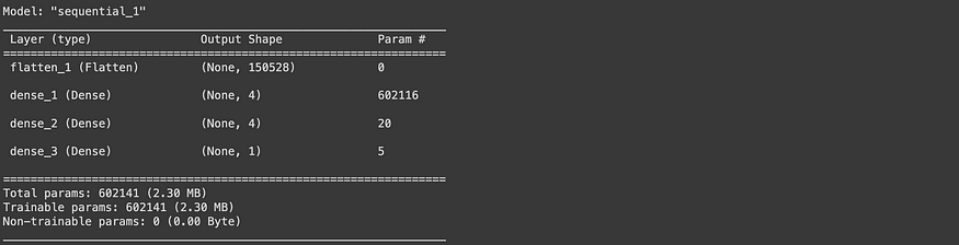
Now, at this stage, I’m adding extra layer to increase complexity of model.
# Set random seed
tf.random.set_seed(42)

# Create a model similar to model_1 but add an extra layer and increase the number of hidden units in each layer
model_3 = tf.keras.Sequential([
  tf.keras.layers.Flatten(input_shape=(224, 224, 3)), # dense layers expect a 1-dimensional vector as input
  tf.keras.layers.Dense(100, activation='relu'), # increase number of neurons from 4 to 100 (for each layer)
  tf.keras.layers.Dense(100, activation='relu'),
  tf.keras.layers.Dense(100, activation='relu'), # add an extra layer
  tf.keras.layers.Dense(1, activation='sigmoid')
])

# Compile the model
model_3.compile(loss='binary_crossentropy',
              optimizer=tf.keras.optimizers.Adam(),
              metrics=["accuracy"])

# Fit the model
history_3 = model_3.fit(train_data,
                        epochs=5,
                        steps_per_epoch=len(train_data),
                        validation_data=valid_data,
                        validation_steps=len(valid_data))

Output:

Epoch 1/5
47/47 [==============================] - 7s 110ms/step - loss: 3.7118 - accuracy: 0.6507 - val_loss: 1.1742 - val_accuracy: 0.7060
Epoch 2/5
47/47 [==============================] - 7s 141ms/step - loss: 1.0191 - accuracy: 0.7273 - val_loss: 0.4365 - val_accuracy: 0.8060
Epoch 3/5
47/47 [==============================] - 7s 140ms/step - loss: 0.7371 - accuracy: 0.7133 - val_loss: 0.7180 - val_accuracy: 0.6380
Epoch 4/5
47/47 [==============================] - 5s 108ms/step - loss: 0.6688 - accuracy: 0.7507 - val_loss: 0.4446 - val_accuracy: 0.7920
Epoch 5/5
47/47 [==============================] - 6s 138ms/step - loss: 0.5615 - accuracy: 0.7620 - val_loss: 0.9812 - val_accuracy: 0.6980
# Check out model_3 architecture
model_3.summary()
- Import and become one with data
# Visualize data (requires function 'view_random_image' above)
plt.figure()
plt.subplot(1, 2, 1)
steak_img = view_random_image("pizza_steak/train/", "steak")
plt.subplot(1, 2, 2)
pizza_img = view_random_image("pizza_steak/train/", "pizza")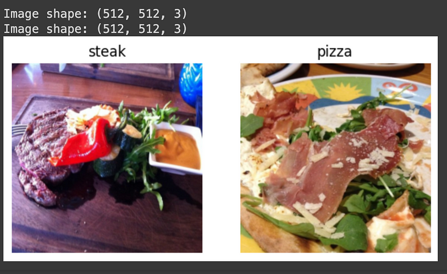
2. Preprocess the data (preparing it for a model)
# Define training and test directory paths
train_dir = "pizza_steak/train/"
test_dir = "pizza_steak/test/"

# Create train and test data generators and rescale the data
from tensorflow.keras.preprocessing.image import ImageDataGenerator
train_datagen = ImageDataGenerator(rescale=1/255.)
test_datagen = ImageDataGenerator(rescale=1/255.)

# Turn it into batches
train_data = train_datagen.flow_from_directory(directory=train_dir,
                                               target_size=(224, 224),
                                               class_mode='binary',
                                               batch_size=32)

test_data = test_datagen.flow_from_directory(directory=test_dir,
                                             target_size=(224, 224),
                                             class_mode='binary',
                                             batch_size=32)

Output:

Found 1500 images belonging to 2 classes.
Found 500 images belonging to 2 classes.
# Get a sample of the training data batch
images, labels = train_data.next() # get the 'next' batch of images/labels
len(images), len(labels)
# (32, 32)
# Get the first two images
images[:2], images[0].shape
[0.7960785 , 0.56078434, 0.27450982],
[0.81568635, 0.54901963, 0.22352943],
...,
[0.23529413, 0.19607845, 0.16078432],
[0.29803923, 0.27058825, 0.2392157 ],
[0.26666668, 0.2509804 , 0.2392157 ]]],
[[[0.38823533, 0.4666667 , 0.36078432],
[0.3921569 , 0.46274513, 0.36078432],
[0.38431376, 0.454902 , 0.36078432],
...,
[0.5294118 , 0.627451 , 0.54509807],
[0.5294118 , 0.627451 , 0.54509807],
[0.5411765 , 0.6392157 , 0.5568628 ]],
[[0.38431376, 0.454902 , 0.3529412 ],
[0.3921569 , 0.46274513, 0.36078432],
[0.39607847, 0.4666667 , 0.37254903],
...,
[0.54509807, 0.6431373 , 0.5686275 ],
[0.5529412 , 0.64705884, 0.58431375],
[0.5647059 , 0.65882355, 0.59607846]],
[[0.3921569 , 0.46274513, 0.36862746],
[0.38431376, 0.454902 , 0.36078432],
[0.41176474, 0.47058827, 0.3803922 ],
...,
[0.5686275 , 0.6745098 , 0.6156863 ],
[0.5647059 , 0.6666667 , 0.6156863 ],
[0.5647059 , 0.6666667 , 0.6156863 ]],
...,
[[0.47058827, 0.5647059 , 0.4784314 ],
[0.48235297, 0.5764706 , 0.4901961 ],
[0.48235297, 0.5803922 , 0.49803925],
...,
[0.39607847, 0.42352945, 0.3019608 ],
[0.37647063, 0.40000004, 0.2901961 ],
[0.3803922 , 0.4039216 , 0.3019608 ]],
[[0.45098042, 0.5529412 , 0.454902 ],
[0.46274513, 0.5647059 , 0.4666667 ],
[0.47058827, 0.5686275 , 0.48235297],
...,
[0.40784317, 0.43137258, 0.32156864],
[0.39607847, 0.41960788, 0.31764707],
[0.38823533, 0.40784317, 0.31764707]],
[[0.47450984, 0.5764706 , 0.4784314 ],
[0.47058827, 0.57254905, 0.47450984],
[0.46274513, 0.5647059 , 0.4666667 ],
...,
[0.4039216 , 0.427451 , 0.31764707],
[0.3921569 , 0.41176474, 0.32156864],
[0.4039216 , 0.42352945, 0.3372549 ]]]], dtype=float32),
(224, 224, 3))# View the first batch of labels
labels
array([1., 1., 0., 1., 0., 0., 0., 1., 0., 1., 0., 0., 1., 0., 0., 0., 1.,
1., 0., 1., 0., 1., 1., 1., 0., 0., 0., 0., 0., 1., 0., 1.],
dtype=float32)3. Creating a model (starting with a baseline)
*Important Explanations**
- Why Three Conv2D Layers?: Using multiple Conv2D layers allows for deeper and more detailed extraction of features in an image. The first layer captures more general features like edges and color transitions, while subsequent layers transform this information into more complex features like patterns and shapes. Three layers offer a balanced choice between model complexity and computational cost.
- Why 10 Filters in Each Layer?: The number of filters determines how many different features the model can detect simultaneously. 10 filters provide a sufficient number to capture a variety of features without overly increasing computational load. As the number of filters increases, the model can learn more features, but also requires more parameters and computation.
- Why Kernel Size of 3?: A kernel_size of 3 means each filter is 3x3 pixels, which is small enough to capture local features while also capturing general features without getting lost in too much detail. The 3x3 size is a common choice as it offers a good balance between detail capture and computational efficiency.
- Why Strides of 1?: strides=1 indicates that the filter moves one pixel at a time, allowing for a detailed traversal over the image and capturing finer features. Larger stride sizes, like 2, would make the filter move faster and capture less detailed features.
- Why ‘Valid’ Padding?: padding=’valid’ means the filter only works on areas where it can fully fit inside the input image, leading to a decrease in input size across layers. Had ‘same’ padding been used, zeroes would be added to the edges of the image to keep the output size the same as the input.
- Why Activation=’ReLU’?: ReLU (Rectified Linear Unit) is an activation function that is linear (unchanged) for positive inputs and zero for negative inputs. It enables fast training of the model and usually yields good results in convolutional neural networks. ReLU allows the network to learn non-linear features, which is essential for complex tasks.
- Why 1 Neuron in Dense Layer and Activation=’Sigmoid’?: The Dense layer, being the output layer of the model, performs the final classification. One neuron is sufficient for binary classification tasks (e.g., yes or no). The activation=’sigmoid’ ensures the output is between 0 and 1, commonly used in binary classification (e.g., determining whether an image belongs to a particular class).
# Create the model (this can be our baseline, a 3 layer Convolutional Neural Network)
model_4 = Sequential([
  Conv2D(filters=10,
         kernel_size=3,
         strides=1,
         padding='valid',
         activation='relu',
         input_shape=(224, 224, 3)), # input layer (specify input shape)
  Conv2D(10, 3, activation='relu'),
  Conv2D(10, 3, activation='relu'),
  Flatten(),
  Dense(1, activation='sigmoid') # output layer (specify output shape)
])- Loss Function (loss=’binary_crossentropy’): The loss function measures how accurate the model’s predictions are. ‘binary_crossentropy’ is commonly used for binary classification tasks. It calculates the difference between the model’s predictions and the actual labels. The model learns to make more accurate predictions by trying to minimize this loss value.
- Optimizer (optimizer=Adam()): The optimizer determines how the model’s weights will be adjusted based on the loss function. The Adam optimizer is widely used because it is generally efficient and effective. Adam dynamically adjusts different learning rates, facilitating faster and more efficient training of the model.
- Metrics (metrics=[‘accuracy’]): Metrics are criteria used to assess the model’s performance. ‘accuracy’ measures the proportion of correct predictions made by the model. During the model’s training, the accuracy value is used to understand how well the model is performing.
If it were a multi-class classification task, a different loss function, like ‘categorical_crossentropy’, might be used. This function is tailored for situations where predictions are to be made across more than two categories.
# Compile the model
model_4.compile(loss='binary_crossentropy',
                optimizer=Adam(),
                metrics=['accuracy'])
Fitting the model
The process of fitting your deep learning model involves setting up how it will progress through each training cycle (epoch) and how it will be tested with validation data. Let’s explain:
- steps_per_epoch Parameter: This specifies the number of batches the model should pass through in each epoch. If your training dataset has 1500 images and each batch contains 32 images, the steps_per_epoch should be equal to 1500/32, which is approximately 47 steps. This setting ensures that the model sees the entire training dataset in each epoch.
- validation_steps Parameter: This indicates the number of batches the model should pass through during validation. If your validation (test) dataset has 500 images and each batch contains 32 images, the validation_steps should be 500/32, which is approximately 16 steps. This ensures the model sees the entire validation dataset and assesses its performance.
- Training the Model: The model_4.fit function initiates the training process of the model. With epochs=5, it is specified that the model will go over the training dataset 5 times. The steps_per_epoch and validation_steps parameters determine how many steps will be taken in each epoch and during validation, respectively. train_data and test_data are the datasets to be used for training and validation, respectively.
- Training History (history_4): The history_4 variable records the model’s performance (accuracy, loss values, etc.) during the training process. This information can be used to analyze how the model developed and performed with specific settings.
# Fit the model
history_4 = model_4.fit(train_data,
                        epochs=5,
                        steps_per_epoch=len(train_data),
                        validation_data=test_data,
                        validation_steps=len(test_data))

Epoch 1/5
47/47 [==============================] - 12s 207ms/step - loss: 0.6666 - accuracy: 0.6900 - val_loss: 0.5516 - val_accuracy: 0.7060
Epoch 2/5
47/47 [==============================] - 8s 165ms/step - loss: 0.4483 - accuracy: 0.7920 - val_loss: 0.3826 - val_accuracy: 0.8440
Epoch 3/5
47/47 [==============================] - 8s 170ms/step - loss: 0.3495 - accuracy: 0.8593 - val_loss: 0.3786 - val_accuracy: 0.8200
Epoch 4/5
47/47 [==============================] - 6s 121ms/step - loss: 0.2472 - accuracy: 0.9127 - val_loss: 0.3891 - val_accuracy: 0.8160
Epoch 5/5
47/47 [==============================] - 6s 118ms/step - loss: 0.1178 - accuracy: 0.9687 - val_loss: 0.5213 - val_accuracy: 0.7920
Evaluating the model
Note1: When a model’s validation loss starts to increase, it’s likely that it’s overfitting the training dataset. This means, it’s learning the patterns in the training dataset too well and thus its ability to generalize to unseen data will be diminished.
Note2: When a model’s validation loss starts to increase, it’s likely that it’s overfitting the training dataset. This means, it’s learning the patterns in the training dataset too well and thus its ability to generalize to unseen data will be diminished.
# Plot the training curves
import pandas as pd
pd.DataFrame(history_4.history).plot(figsize=(10, 7));
# Plot the validation and training data separately
def plot_loss_curves(history):
  """
  Returns separate loss curves for training and validation metrics.
  """
  loss = history.history['loss']
  val_loss = history.history['val_loss']

  accuracy = history.history['accuracy']
  val_accuracy = history.history['val_accuracy']

  epochs = range(len(history.history['loss']))

  # Plot loss
  plt.plot(epochs, loss, label='training_loss')
  plt.plot(epochs, val_loss, label='val_loss')
  plt.title('Loss')
  plt.xlabel('Epochs')
  plt.legend()

  # Plot accuracy
  plt.figure()
  plt.plot(epochs, accuracy, label='training_accuracy')
  plt.plot(epochs, val_accuracy, label='val_accuracy')
  plt.title('Accuracy')
  plt.xlabel('Epochs')
  plt.legend();

# Check out our model's architecture
model_4.summary()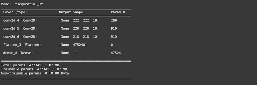
Adjusting the model parameters
- Three Stages of Machine Learning Model Development:
- Establishing a Baseline: The first step involves creating a simple model to determine its initial performance, which serves as a reference point for future improvements.
- Exceeding Baseline with Overfitting: Making the model more complex to achieve higher performance on training data often leads to overfitting, where the model becomes too tailored to the training data and loses its ability to generalize.
- Reducing Overfitting: Adjustments are made to balance the model’s performance on training data and its ability to perform well on unseen data.
2. Importance of Reducing Overfitting: If a model performs exceptionally well on training data but poorly on new, unseen data, it is not very useful for real-world applications. For instance, in a pizza vs. steak classifier application, if the model excels on training data but performs poorly when users try it with their own images, it does not provide a good user experience.
3. Creating a New Model (model_5): The structure of model_5 is similar to model_4, but with a MaxPool2D layer added after each Conv2D layer. The MaxPool2D layers help the model learn more general features and reduce overfitting by halving the number of features. The model consists of 3 Conv2D layers, each followed by a MaxPool2D layer, a Flatten layer, and a final output Dense(1, activation=’sigmoid’) layer. This approach aids in learning more general features and performing better on new data.
4. First Model Structure: The initial model follows a modified basic CNN structure with an Input -> Conv layers + ReLU layers (non-linearities) + Max Pooling layers -> Fully connected (dense) Output layer. It is built with the same structure as model_4 but includes a MaxPool2D() layer after each convolutional layer to help in reducing overfitting and improving generalization on real-world data.
# Create the model (this can be our baseline, a 3 layer Convolutional Neural Network)
model_5 = Sequential([
  Conv2D(10, 3, activation='relu', input_shape=(224, 224, 3)),
  MaxPool2D(pool_size=2), # reduce number of features by half
  Conv2D(10, 3, activation='relu'),
  MaxPool2D(),
  Conv2D(10, 3, activation='relu'),
  MaxPool2D(),
  Flatten(),
  Dense(1, activation='sigmoid')
])

# Compile model (same as model_4)
model_5.compile(loss='binary_crossentropy',
                optimizer=Adam(),
                metrics=['accuracy'])

# Fit the model
history_5 = model_5.fit(train_data,
                        epochs=5,
                        steps_per_epoch=len(train_data),
                        validation_data=test_data,
                        validation_steps=len(test_data))

Output:

Epoch 1/5
47/47 [==============================] - 14s 243ms/step - loss: 0.6675 - accuracy: 0.5813 - val_loss: 0.5527 - val_accuracy: 0.7660
Epoch 2/5
47/47 [==============================] - 9s 192ms/step - loss: 0.5058 - accuracy: 0.7580 - val_loss: 0.4207 - val_accuracy: 0.8280
Epoch 3/5
47/47 [==============================] - 5s 113ms/step - loss: 0.4503 - accuracy: 0.7973 - val_loss: 0.4081 - val_accuracy: 0.8240
Epoch 4/5
47/47 [==============================] - 6s 123ms/step - loss: 0.4253 - accuracy: 0.8087 - val_loss: 0.3842 - val_accuracy: 0.8300
Epoch 5/5
47/47 [==============================] - 5s 113ms/step - loss: 0.4042 - accuracy: 0.8260 - val_loss: 0.3978 - val_accuracy: 0.8180
Okay, it looks like our model with max pooling (model_5) is performing worse on the training set but better on the validation set. Before we checkout its training curves, let’s check out its architecture.
# Check out the model architecture
model_5.summary()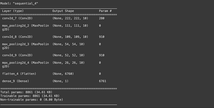
MaxPooling2D layers significantly affect the output dimensions of the feature maps generated by Conv2D layers in a deep learning model. Let’s explain how they alter the output dimensions:
Effect of MaxPooling2D Layers: Each MaxPooling2D layer reduces the dimensions of the output from the previous Conv2D layer by half. This reduction is dependent on the pool_size parameter. When using MaxPool2D(pool_size=2), the number of features in each dimension is halved. For instance, a feature map of size 224x224 becomes 112x112 after passing through MaxPooling. The MaxPooling layer captures the most significant parts of the features detected by each filter and discards the rest, enabling the model to focus only on the most important features.
MaxPooling and Model’s Learning Capability: A larger pool_size compresses the features more, but an excessively large pool_size might prevent the model from learning enough features. A balanced pool_size selection allows the model to learn adequate features while reducing the computational burden.
Reduction in Total Trainable Parameters: MaxPooling substantially decreases the total number of trainable parameters in the model. For example, while model_5 has a total of 8,861 trainable parameters, model_4 has 477,431. This reduction results from MaxPooling layers decreasing the size of feature maps, thereby transmitting less data to subsequent layers.
Analysis of Loss Curves: The loss curves during the model’s training process indicate how the model performs on training and validation data. These curves are used to assess whether the model is overfitting and to evaluate its generalization ability.
These characteristics demonstrate that MaxPooling layers help in making the model more efficient while maintaining a balance in learning sufficient features. This contributes to enhancing the model’s overall performance and its ability to generalize on data.
# Plot loss curves of model_5 results
plot_loss_curves(history_5)

Yes, observing the training and validation loss curves converging is a sign of the model’s improving ability to generalize. However, if the validation loss begins to increase towards the end of training, it could be a sign of overfitting. In this case, other methods may need to be tried to prevent overfitting. One such method is ‘data augmentation.’
What is Data Augmentation?
Data augmentation is the process of artificially altering existing training data to increase its diversity. This helps reduce overfitting by enabling the model to adapt to a wider range of data. Typical data augmentation techniques include image rotation, scaling, flipping horizontally or vertically, and color changes.
How is Data Augmentation Applied?
Data augmentation can be implemented using the ImageDataGenerator class. This class allows for various transformations to be applied while loading training data into the model. You can apply data augmentation by creating a new instance of ImageDataGenerator and defining data augmentation parameters.
Note: Data augmentation is usually only performed on the training data. Using the built-in data augmentation parameters of ImageDataGenerator, our images remain as they are in the directories but are randomly manipulated when loaded into the model.
# Create ImageDataGenerator training instance with data augmentation
train_datagen_augmented = ImageDataGenerator(rescale=1/255.,
                                             rotation_range=20, # rotate the image slightly between 0 and 20 degrees (note: this is an int not a float)
                                             shear_range=0.2, # shear the image
                                             zoom_range=0.2, # zoom into the image
                                             width_shift_range=0.2, # shift the image width ways
                                             height_shift_range=0.2, # shift the image height ways
                                             horizontal_flip=True) # flip the image on the horizontal axis

# Create ImageDataGenerator training instance without data augmentation
train_datagen = ImageDataGenerator(rescale=1/255.)

# Create ImageDataGenerator test instance without data augmentation
test_datagen = ImageDataGenerator(rescale=1/255.)
Creating a Training Dataset with Data Augmentation: Data augmentation is defined using the ImageDataGenerator class. The images’ pixel values are scaled between 0 and 1 using rescale=1/255. The images are randomly rotated between 0 and 20 degrees with rotation_range=20. Shear, zoom, and shift transformations are applied with shear_range=0.2, zoom_range=0.2, width_shift_range=0.2, height_shift_range=0.2. Horizontal flipping is enabled with horizontal_flip=True. These processes help train the model on more diverse images, improving its generalization capability.
Creating Training and Test Datasets without Data Augmentation: Additionally, training and test datasets without data augmentation are also created. These datasets maintain the original images, applying only the rescale operation.
Loading Datasets: The datasets are loaded using the flow_from_directory method. For training and test datasets, the parameters target_size=(224, 224) and batch_size=32 are set. The parameter class_mode=’binary’ indicates a binary classification problem. For training sets, shuffle=False is specified, though typically, shuffling the data is preferred.
Results: Both training datasets (with and without augmentation) contain 1500 images and are divided into two classes. The test dataset includes 500 unaltered images, also divided into two classes.
# Import data and augment it from training directory
print("Augmented training images:")
train_data_augmented = train_datagen_augmented.flow_from_directory(train_dir,
                                                                   target_size=(224, 224),
                                                                   batch_size=32,
                                                                   class_mode='binary',
                                                                   shuffle=False) # Don't shuffle for demonstration purposes, usually a good thing to shuffle

# Create non-augmented data batches
print("Non-augmented training images:")
train_data = train_datagen.flow_from_directory(train_dir,
                                               target_size=(224, 224),
                                               batch_size=32,
                                               class_mode='binary',
                                               shuffle=False) # Don't shuffle for demonstration purposes

print("Unchanged test images:")
test_data = test_datagen.flow_from_directory(test_dir,
                                             target_size=(224, 224),
                                             batch_size=32,
                                             class_mode='binary')

Output:

Augmented training images:
Found 1500 images belonging to 2 classes.
Non-augmented training images:
Found 1500 images belonging to 2 classes.
Unchanged test images:
Found 500 images belonging to 2 classes.
# Get data batch samples
images, labels = train_data.next()
augmented_images, augmented_labels = train_data_augmented.next() # Note: labels aren't augmented, they stay the same
# Show original image and augmented image
random_number = random.randint(0, 31) # we're making batches of size 32, so we'll get a random instance
plt.imshow(images[random_number])
plt.title(f"Original image")
plt.axis(False)
plt.figure()
plt.imshow(augmented_images[random_number])
plt.title(f"Augmented image")
plt.axis(False);
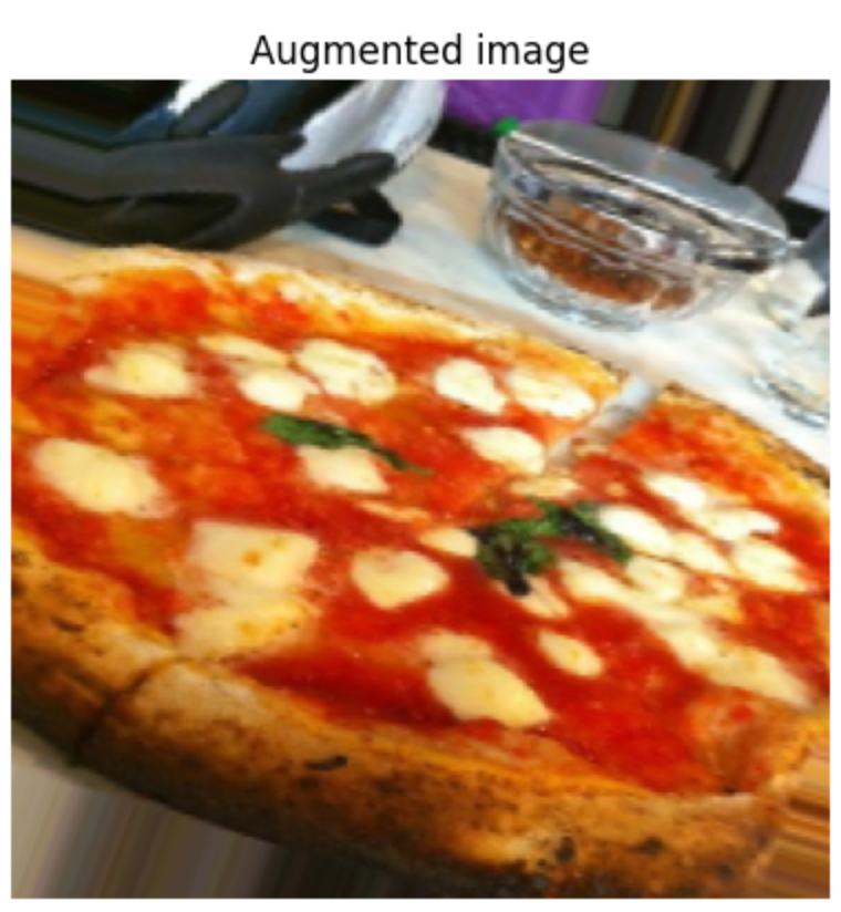
Data Augmentation Application: Data augmentation is implemented by adding artificial transformations to the training dataset. These transformations can include rotating, scaling, shifting, shearing, and flipping images. These transformations enable the model to learn from a broader range of data, preventing overfitting to the training data.
Amount of Data Augmentation: Deciding how much data augmentation to apply is often a trial-and-error process. You can develop a strategy by reviewing the options in the ImageDataGenerator class and considering which types of data augmentations might benefit your model based on your use case. Excessive data augmentation can lead to the model losing essential features it needs to learn, so a balanced approach is important.
Retraining the Model: Retraining the model on augmented data is a good way to see how it affects the model’s performance. This is assessed by examining the training and validation loss curves and accuracy rates of the model.
For this process, we’ll use the same model as “model_5.” This means we’ll be retraining “model_5” with the newly augmented data to observe any improvements or changes in its performance. This approach allows us to directly compare the effects of data augmentation on the same model structure, providing clear insights into the impact of these enhancements on the model’s ability to generalize and reduce overfitting.
# Create the model (same as model_5)
model_6 = Sequential([
  Conv2D(10, 3, activation='relu', input_shape=(224, 224, 3)),
  MaxPool2D(pool_size=2), # reduce number of features by half
  Conv2D(10, 3, activation='relu'),
  MaxPool2D(),
  Conv2D(10, 3, activation='relu'),
  MaxPool2D(),
  Flatten(),
  Dense(1, activation='sigmoid')
])

# Compile the model
model_6.compile(loss='binary_crossentropy',
                optimizer=Adam(),
                metrics=['accuracy'])

# Fit the model
history_6 = model_6.fit(train_data_augmented, # changed to augmented training data
                        epochs=5,
                        steps_per_epoch=len(train_data_augmented),
                        validation_data=test_data,
                        validation_steps=len(test_data))

Epoch 1/5
47/47 [==============================] - 24s 481ms/step - loss: 0.8942 - accuracy: 0.4160 - val_loss: 0.6998 - val_accuracy: 0.5000
Epoch 2/5
47/47 [==============================] - 23s 482ms/step - loss: 0.6955 - accuracy: 0.4700 - val_loss: 0.6813 - val_accuracy: 0.5340
Epoch 3/5
47/47 [==============================] - 22s 459ms/step - loss: 0.6861 - accuracy: 0.5713 - val_loss: 0.6921 - val_accuracy: 0.5060
Epoch 4/5
47/47 [==============================] - 26s 566ms/step - loss: 0.6854 - accuracy: 0.5720 - val_loss: 0.6479 - val_accuracy: 0.6640
Epoch 5/5
47/47 [==============================] - 23s 489ms/step - loss: 0.6798 - accuracy: 0.5587 - val_loss: 0.6281 - val_accuracy: 0.6480
Low Performance on Training Dataset: One reason for the model’s initially low performance on the training set could be the use of the shuffle=False option when creating train_data_augmented. shuffle=False leads to the model seeing batches of images from only one class at a time. For instance, if the “pizza” class is first, the model initially trains only on pizza images. This situation prevents the model from learning the characteristics of both classes in a balanced way during training.
Stable Performance on Validation Dataset: Since the validation dataset contains shuffled data, the model exhibits a more balanced and stable performance on it. This allows the model to more evenly assess the characteristics of both classes.
Importance of Shuffling: Using shuffle=True in future trainings could resolve this issue. This setting ensures that each batch contains samples from both classes, aiding the model in learning the features of both classes more evenly.
Training Duration with Augmented Data: It’s normal for each epoch to take longer when data augmentation is applied. This is due to the ImageDataGenerator performing real-time data augmentation processes as it loads data into the model. The advantage of this method is that the original images remain unchanged. The disadvantage is the longer duration of data loading.
Speeding Up Data Processing: To accelerate dataset processing time, it might be beneficial to look into TensorFlow’s parallel reading and buffered prefetching options.
In conclusion, it’s important to use the data shuffling setting (shuffle=True) to ensure your model effectively learns from the training data. Additionally, remember that applying data augmentation practices will extend the training time, and this should be considered in your planning.
# Check model's performance history training on augmented data
plot_loss_curves(history_6)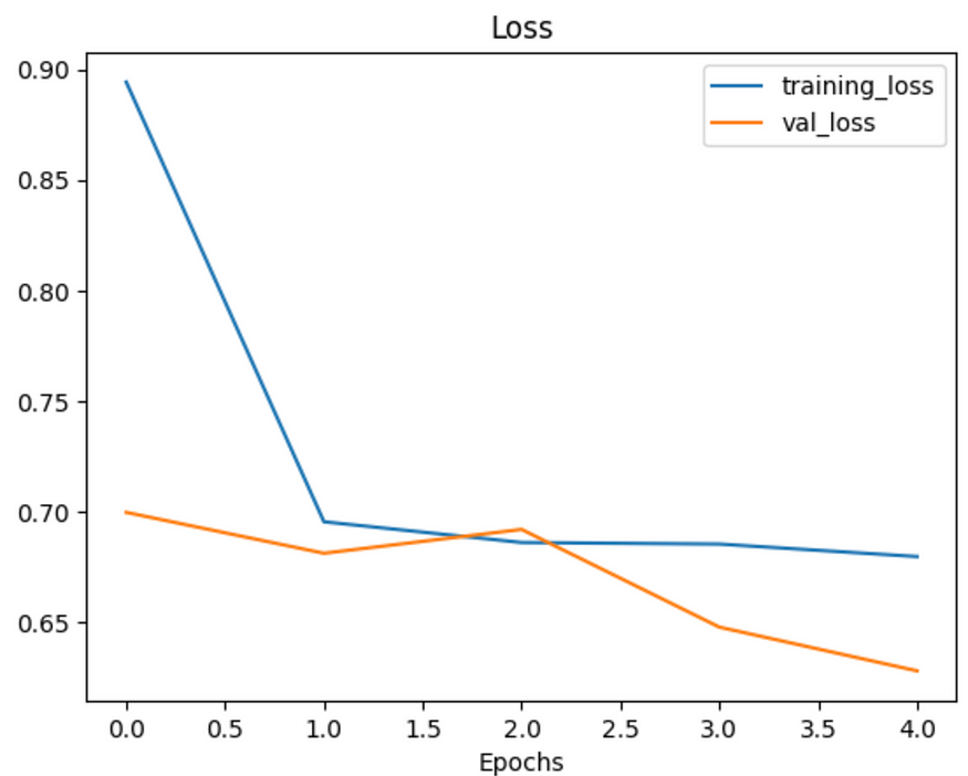

Shuffling Augmented Training Data: Shuffling the augmented training data can have a significant impact on the training process and the behavior of the loss curve. Let’s explore this aspect:
Impact of Shuffling on Learning Dynamics: Shuffling the data ensures that each batch during training is a random mix of all the classes and variations in the dataset. This randomness can help the model learn more general features and prevent it from overfitting to specific sequences of data.
Effect on Loss Curve: When the augmented training data is shuffled, the model is exposed to a more diverse set of data in each batch. This diversity can lead to a more stable and consistent learning process, potentially smoothing out the fluctuations in the loss curve.
Experimenting with Shuffling: By shuffling the augmented data, you might notice a change in the training dynamics. The loss curve could become more stable, indicating a more uniform learning process across different batches. However, it’s also possible that the curve remains somewhat volatile due to the inherent diversity introduced by data augmentation.
Balancing Augmentation and Shuffling: While data augmentation introduces variety, shuffling ensures that this variety is evenly distributed throughout the training process. The combination of both can lead to more robust learning but might require adjustments in other training parameters like learning rate, batch size, or the choice of the optimizer, as mentioned earlier.
In summary, shuffling the augmented training data can be a crucial step in ensuring that the model is not biased towards specific sequences or types of data, leading to better generalization and potentially smoother loss curves. It’s an experiment worth conducting to see how it affects your specific model and dataset.
# Import data and augment it from directories
train_data_augmented_shuffled = train_datagen_augmented.flow_from_directory(train_dir,
                                                                            target_size=(224, 224),
                                                                            batch_size=32,
                                                                            class_mode='binary',
                                                                            shuffle=True) # Shuffle data (default)

Output:
Found 1500 images belonging to 2 classes.

# Create the model (same as model_5 and model_6)
model_7 = Sequential([
  Conv2D(10, 3, activation='relu', input_shape=(224, 224, 3)),
  MaxPool2D(),
  Conv2D(10, 3, activation='relu'),
  MaxPool2D(),
  Conv2D(10, 3, activation='relu'),
  MaxPool2D(),
  Flatten(),
  Dense(1, activation='sigmoid')
])

# Compile the model
model_7.compile(loss='binary_crossentropy',
                optimizer=Adam(),
                metrics=['accuracy'])

# Fit the model
history_7 = model_7.fit(train_data_augmented_shuffled, # now the augmented data is shuffled
                        epochs=5,
                        steps_per_epoch=len(train_data_augmented_shuffled),
                        validation_data=test_data,
                        validation_steps=len(test_data))

Epoch 1/5
47/47 [==============================] - 23s 458ms/step - loss: 0.6510 - accuracy: 0.6227 - val_loss: 0.4911 - val_accuracy: 0.7980
Epoch 2/5
47/47 [==============================] - 23s 492ms/step - loss: 0.5498 - accuracy: 0.7440 - val_loss: 0.4312 - val_accuracy: 0.8260
Epoch 3/5
47/47 [==============================] - 22s 461ms/step - loss: 0.5358 - accuracy: 0.7467 - val_loss: 0.4361 - val_accuracy: 0.8260
Epoch 4/5
47/47 [==============================] - 23s 499ms/step - loss: 0.5071 - accuracy: 0.7673 - val_loss: 0.3832 - val_accuracy: 0.8480
Epoch 5/5
47/47 [==============================] - 27s 574ms/step - loss: 0.5062 - accuracy: 0.7580 - val_loss: 0.4974 - val_accuracy: 0.7480
# Check model's performance history training on augmented data
plot_loss_curves(history_7)

Shuffling the Training Dataset (shuffle=True) can significantly impact the training process of a model. Here are the reasons for the improvement in performance and the smoothing of the loss curves for model_7:
Training Data Shuffling: The shuffle=True parameter, used with the flow_from_directory method, enables the shuffling of training data. This ensures that the model encounters a mix of both pizza and steak images in each batch. The model learns from examples of both classes, which helps it perform more balanced across both categories.
Improved Training Performance: Model_7 has shown immediate improvement in its performance on the training dataset. This indicates that the model is learning the characteristics of both classes more quickly and effectively. Shuffled data exposes the model to a more diverse set of examples during training, enhancing its learning experience.
Smoother Loss Curves: The loss curves of the model trained with the shuffled dataset (model_7) appear smoother compared to the model trained without shuffling (model_6). Shuffled data ensures that the model encounters different examples at each step, making the learning process more consistent and stable.
In summary, shuffling the training data (shuffle=True) helps in presenting a more diverse and balanced view of the dataset to the model during training. This not only aids in quicker and more effective learning but also leads to smoother loss curves, indicating a more stable and consistent training process. Such improvements are crucial for developing a model that generalizes well and performs consistently on new, unseen data.
Repeating until satisfied!
Adjusting Model Layers: You can add more convolutional layers to your model. This can help the model learn more complex features.
Increasing the Number of Filters: Increase the number of filters (feature extractors) in existing layers (e.g., from 10 to 32, 64, or 128). Determining the optimal number of filters is usually done through trial and error.
Training for a Longer Duration: Training your model for more epochs can lead to better learning.
Finding the Ideal Learning Rate: Identifying the learning rate at which your model performs best can increase the efficiency of the training.
Acquiring More Data: Providing more training data to your model can enhance its ability to generalize.
Using Transfer Learning: You can improve your model by utilizing what another image model has learned and adapting it to your use case. This is particularly effective for large and complex datasets.
These adjustments, except for the last two points, are typically referred to as “hyperparameter tuning” in the model development process. Hyperparameter tuning is like adjusting the settings of your oven while cooking your favorite meal: the oven does most of the work, but you can help by slightly tweaking the settings.
Now, let’s circle back to the starting point and retry your original model (model_1 or the TinyVGG architecture from CNN Explainer). This offers a good opportunity to review your starting point and assess the progress you’ve made so far.
# Create a CNN model (same as Tiny VGG but for binary classification - https://poloclub.github.io/cnn-explainer/ )
model_8 = Sequential([
  Conv2D(10, 3, activation='relu', input_shape=(224, 224, 3)), # same input shape as our images
  Conv2D(10, 3, activation='relu'),
  MaxPool2D(),
  Conv2D(10, 3, activation='relu'),
  Conv2D(10, 3, activation='relu'),
  MaxPool2D(),
  Flatten(),
  Dense(1, activation='sigmoid')
])

# Compile the model
model_8.compile(loss="binary_crossentropy",
                optimizer=tf.keras.optimizers.Adam(),
                metrics=["accuracy"])

# Fit the model
history_8 = model_8.fit(train_data_augmented_shuffled,
                        epochs=5,
                        steps_per_epoch=len(train_data_augmented_shuffled),
                        validation_data=test_data,
                        validation_steps=len(test_data))


Epoch 1/5
47/47 [==============================] - 26s 528ms/step - loss: 0.6772 - accuracy: 0.5740 - val_loss: 0.5652 - val_accuracy: 0.7320
Epoch 2/5
47/47 [==============================] - 25s 545ms/step - loss: 0.5459 - accuracy: 0.7313 - val_loss: 0.3953 - val_accuracy: 0.8340
Epoch 3/5
47/47 [==============================] - 22s 462ms/step - loss: 0.4735 - accuracy: 0.7827 - val_loss: 0.3498 - val_accuracy: 0.8600
Epoch 4/5
47/47 [==============================] - 29s 611ms/step - loss: 0.4443 - accuracy: 0.8020 - val_loss: 0.3524 - val_accuracy: 0.8520
Epoch 5/5
47/47 [==============================] - 24s 503ms/step - loss: 0.4526 - accuracy: 0.7867 - val_loss: 0.3103 - val_accuracy: 0.8620
Note: It’s noticed we used some slightly different code to build model_8 as compared to model_1. This is because of the imports we did before, such as from tensorflow.keras.layers import Conv2D reduce the amount of code we had to write. Although the code is different, the architectures are the same.
# Check model_1 architecture (same as model_8)
model_1.summary()
# Check model_8 architecture (same as model_1)
model_8.summary()
# Check out the TinyVGG model performance
plot_loss_curves(history_8)

# How does this training curve look compared to the one above?
plot_loss_curves(history_1)

Making a prediction with our trained model
To test it out, we’ll upload a couple of our own images and see how the model goes. Let’s remind us of classnames and view the image to test.
# View our example image
!wget https://raw.githubusercontent.com/mrdbourke/tensorflow-deep-learning/main/images/03-steak.jpeg
steak = mpimg.imread("03-steak.jpeg")
plt.imshow(steak)
plt.axis(False);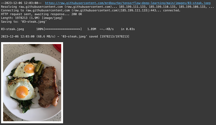
# Check the shape of our image
steak.shape
#(4032, 3024, 3)
Since our model takes in images of shapes (224, 224, 3), we’ve got to reshape our custom image to use it with our model.
To do so, we can import and decode our image using tf.io.read_file (for readining files) and tf.image (for resizing our image and turning it into a tensor).
Note: For model to make predictions on unseen data, for example, your own custom images, the custom image has to be in the same shape as your model has been trained on. In more general terms, to make predictions on custom data it has to be in the same form that your model has been trained on.
# Create a function to import an image and resize it to be able to be used with our model
def load_and_prep_image(filename, img_shape=224):
  """
  Reads an image from filename, turns it into a tensor
  and reshapes it to (img_shape, img_shape, colour_channel).
  """
  # Read in target file (an image)
  img = tf.io.read_file(filename)

  # Decode the read file into a tensor & ensure 3 colour channels
  # (our model is trained on images with 3 colour channels and sometimes images have 4 colour channels)
  img = tf.image.decode_image(img, channels=3)

  # Resize the image (to the same size our model was trained on)
  img = tf.image.resize(img, size = [img_shape, img_shape])

  # Rescale the image (get all values between 0 and 1)
  img = img/255.
  return img


# Load in and preprocess our custom image
steak = load_and_prep_image("03-steak.jpeg")
steak

Output:
<tf.Tensor: shape=(224, 224, 3), dtype=float32, numpy=
array([[[0.6377451 , 0.6220588 , 0.57892156],
        [0.6504902 , 0.63186276, 0.5897059 ],
        [0.63186276, 0.60833335, 0.5612745 ],
        ...,
        [0.52156866, 0.05098039, 0.09019608],
        [0.49509802, 0.04215686, 0.07058824],
        [0.52843136, 0.07745098, 0.10490196]],

       [[0.6617647 , 0.6460784 , 0.6107843 ],
        [0.6387255 , 0.6230392 , 0.57598037],
        [0.65588236, 0.63235295, 0.5852941 ],
        ...,
        [0.5352941 , 0.06862745, 0.09215686],
        [0.529902  , 0.05931373, 0.09460784],
        [0.5142157 , 0.05539216, 0.08676471]],

       [[0.6519608 , 0.6362745 , 0.5892157 ],
        [0.6392157 , 0.6137255 , 0.56764704],
        [0.65637255, 0.6269608 , 0.5828431 ],
        ...,
        [0.53137255, 0.06470589, 0.08039216],
        [0.527451  , 0.06862745, 0.1       ],
        [0.52254903, 0.05196078, 0.0872549 ]],

       ...,

       [[0.49313724, 0.42745098, 0.31029412],
        [0.05441177, 0.01911765, 0.        ],
        [0.2127451 , 0.16176471, 0.09509804],
        ...,
        [0.6132353 , 0.59362745, 0.57009804],
        [0.65294117, 0.6333333 , 0.6098039 ],
        [0.64166665, 0.62990195, 0.59460783]],

       [[0.65392154, 0.5715686 , 0.45      ],
        [0.6367647 , 0.54656863, 0.425     ],
        [0.04656863, 0.01372549, 0.        ],
        ...,
        [0.6372549 , 0.61764705, 0.59411764],
        [0.63529414, 0.6215686 , 0.5892157 ],
        [0.6401961 , 0.62058824, 0.59705883]],

       [[0.1       , 0.05539216, 0.        ],
        [0.48333332, 0.40882352, 0.29117647],
        [0.65      , 0.5686275 , 0.44019607],
        ...,
        [0.6308824 , 0.6161765 , 0.5808824 ],
        [0.6519608 , 0.63186276, 0.5901961 ],
        [0.6338235 , 0.6259804 , 0.57892156]]], dtype=float32)>
Before that, there’s a problem… Although our image is in the same shape as the images our model has been trained on, we’re still missing a dimension. Remember how our model was trained in batches? Well, the batch size becomes the first dimension.
So in reality, our model was trained on data in the shape of (batch_size, 224, 224, 3). We can fix this by adding an extra to our custom image tensor using tf.expand_dims.
# Add an extra axis
print(f"Shape before new dimension: {steak.shape}")
steak = tf.expand_dims(steak, axis=0) # add an extra dimension at axis 0
#steak = steak[tf.newaxis, ...] # alternative to the above, '...' is short for 'every other dimension'
print(f"Shape after new dimension: {steak.shape}")
steak
Our custom image has a batch size of 1! Let’s make a prediction on it.
# Make a prediction on custom image tensor
pred = model_8.predict(steak)
pred


1/1 [==============================] - 0s 174ms/step
array([[0.69249856]], dtype=float32)
Ahh, the predictions come out in prediction probability form. In other words, this means how likely the image is to be one class or another.
Since we’re working with a binary classification problem, if the prediction probability is over 0.5, according to the model, the prediction is most likely to be the postive class (class 1). And if the prediction probability is under 0.5, according to the model, the predicted class is most likely to be the negative class (class 0).
Note: The 0.5 cutoff can be adjusted to your liking. For example, you could set the limit to be 0.8 and over for the positive class and 0.2 for the negative class. However, doing this will almost always change your model’s performance metrics so be sure to make sure they change in the right direction. But saying positive and negative class doesn’t make much sense when we’re working with pizza 🍕 and steak 🥩… So let’s write a little function to convert predictions into their class names and then plot the target image.
# Remind ourselves of our class names
class_names
#array(['pizza', 'steak'], dtype='<U5')

# We can index the predicted class by rounding the prediction probability
pred_class = class_names[int(tf.round(pred)[0][0])]
pred_class
#steak
def pred_and_plot(model, filename, class_names):
"""
Imports an image located at filename, makes a prediction on it with
a trained model and plots the image with the predicted class as the title.
"""
# Import the target image and preprocess it
img = load_and_prep_image(filename)
# Make a prediction
pred = model.predict(tf.expand_dims(img, axis=0))
# Get the predicted class
pred_class = class_names[int(tf.round(pred)[0][0])]
# Plot the image and predicted class
plt.imshow(img)
plt.title(f"Prediction: {pred_class}")
plt.axis(False);
# Test our model on a custom image
pred_and_plot(model_8, "03-steak.jpeg", class_names)
# Download another test image and make a prediction on it
!wget https://raw.githubusercontent.com/mrdbourke/tensorflow-deep-learning/main/images/03-pizza-dad.jpeg
pred_and_plot(model_8, "03-pizza-dad.jpeg", class_names)
MULTICLASS CLASSIFICATION
- Become one with the data (visualize, visualize, visualize…) -Preprocess the data (prepare it for a model)
- -Create a model (start with a baseline) -Fit the model -Evaluate the model
- -Adjust different parameters and improve model (try to beat your baseline)
- -Repeat until satisfied
- Import and become one with the data
Again, we’ve got a subset of the Food101 dataset. In addition to the pizza and steak images, we’ve pulled out another eight classes.
import zipfile

# Download zip file of 10_food_classes images
# See how this data was created - https://github.com/mrdbourke/tensorflow-deep-learning/blob/main/extras/image_data_modification.ipynb
!wget https://storage.googleapis.com/ztm_tf_course/food_vision/10_food_classes_all_data.zip

# Unzip the downloaded file
zip_ref = zipfile.ZipFile("10_food_classes_all_data.zip", "r")
zip_ref.extractall()
zip_ref.close()


--2023-12-06 12:06:40--  https://storage.googleapis.com/ztm_tf_course/food_vision/10_food_classes_all_data.zip
Resolving storage.googleapis.com (storage.googleapis.com)... 108.177.96.207, 108.177.119.207, 108.177.127.207, ...
Connecting to storage.googleapis.com (storage.googleapis.com)|108.177.96.207|:443... connected.
HTTP request sent, awaiting response... 200 OK
Length: 519183241 (495M) [application/zip]
Saving to: ‘10_food_classes_all_data.zip’

10_food_classes_all 100%[===================>] 495.13M  40.0MB/s    in 13s

2023-12-06 12:06:53 (38.2 MB/s) - ‘10_food_classes_all_data.zip’ saved [519183241/519183241]
import os
# Walk through 10_food_classes directory and list number of files
for dirpath, dirnames, filenames in os.walk("10_food_classes_all_data"):
print(f"There are {len(dirnames)} directories and {len(filenames)} images in '{dirpath}'.")
There are 2 directories and 0 images in '10_food_classes_all_data'.
There are 10 directories and 0 images in '10_food_classes_all_data/test'.
There are 0 directories and 250 images in '10_food_classes_all_data/test/sushi'.
There are 0 directories and 250 images in '10_food_classes_all_data/test/fried_rice'.
There are 0 directories and 250 images in '10_food_classes_all_data/test/pizza'.
There are 0 directories and 250 images in '10_food_classes_all_data/test/ramen'.
There are 0 directories and 250 images in '10_food_classes_all_data/test/grilled_salmon'.
There are 0 directories and 250 images in '10_food_classes_all_data/test/chicken_wings'.
There are 0 directories and 250 images in '10_food_classes_all_data/test/hamburger'.
There are 0 directories and 250 images in '10_food_classes_all_data/test/ice_cream'.
There are 0 directories and 250 images in '10_food_classes_all_data/test/chicken_curry'.
There are 0 directories and 250 images in '10_food_classes_all_data/test/steak'.
There are 10 directories and 0 images in '10_food_classes_all_data/train'.
There are 0 directories and 750 images in '10_food_classes_all_data/train/sushi'.
There are 0 directories and 750 images in '10_food_classes_all_data/train/fried_rice'.
There are 0 directories and 750 images in '10_food_classes_all_data/train/pizza'.
There are 0 directories and 750 images in '10_food_classes_all_data/train/ramen'.
There are 0 directories and 750 images in '10_food_classes_all_data/train/grilled_salmon'.
There are 0 directories and 750 images in '10_food_classes_all_data/train/chicken_wings'.
There are 0 directories and 750 images in '10_food_classes_all_data/train/hamburger'.
There are 0 directories and 750 images in '10_food_classes_all_data/train/ice_cream'.
There are 0 directories and 750 images in '10_food_classes_all_data/train/chicken_curry'.
There are 0 directories and 750 images in '10_food_classes_all_data/train/steak'.
[ ]train_dir = "10_food_classes_all_data/train/"
test_dir = "10_food_classes_all_data/test/"
# Get the class names for our multi-class dataset
import pathlib
import numpy as np
data_dir = pathlib.Path(train_dir)
class_names = np.array(sorted([item.name for item in data_dir.glob('*')]))
print(class_names)
['chicken_curry' 'chicken_wings' 'fried_rice' 'grilled_salmon' 'hamburger'
'ice_cream' 'pizza' 'ramen' 'steak' 'sushi']
# View a random image from the training dataset
import random
img = view_random_image(target_dir=train_dir,
target_class=random.choice(class_names)) # get a random class name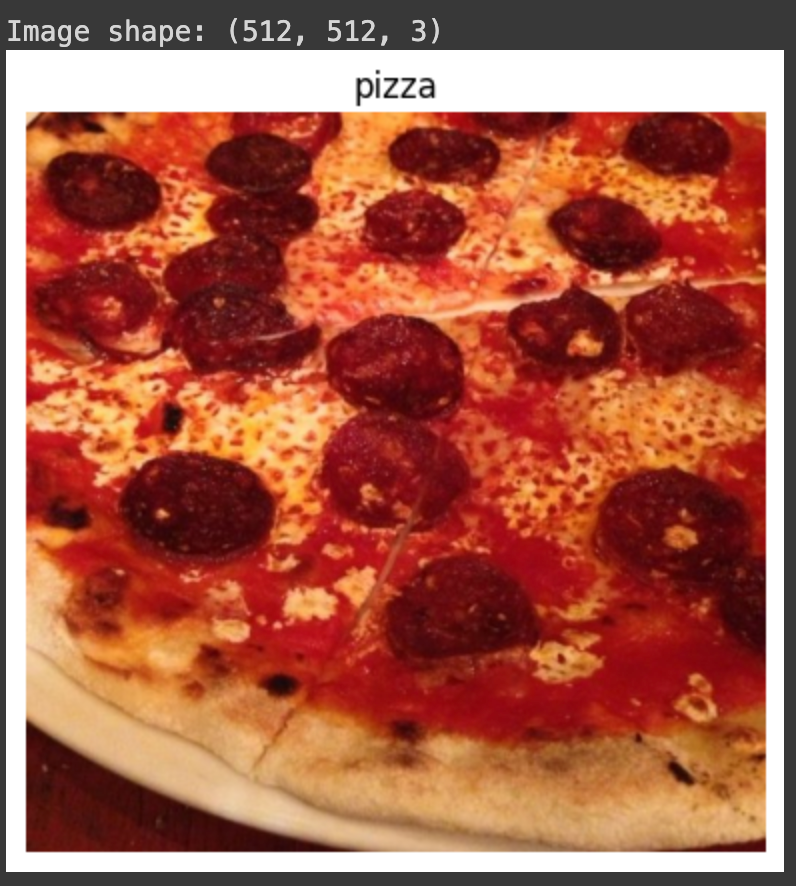
2. Preprocess the data (prepare it for a model)
After going through a handful of images (it’s good to visualize at least 10–100 different examples), it looks like our data directories are setup correctly.
from tensorflow.keras.preprocessing.image import ImageDataGenerator

# Rescale the data and create data generator instances
train_datagen = ImageDataGenerator(rescale=1/255.)
test_datagen = ImageDataGenerator(rescale=1/255.)

# Load data in from directories and turn it into batches
train_data = train_datagen.flow_from_directory(train_dir,
                                               target_size=(224, 224),
                                               batch_size=32,
                                               class_mode='categorical') # changed to categorical

test_data = train_datagen.flow_from_directory(test_dir,
                                              target_size=(224, 224),
                                              batch_size=32,
                                              class_mode='categorical')

#Found 7500 images belonging to 10 classes.
#Found 2500 images belonging to 10 classes.
Changing the Class Mode: When moving from binary classification (where class_mode=’binary’ was used) to a scenario with 10 different food classes, setting class_mode to ‘categorical’ is appropriate. This setting allows the model to classify among multiple classes, which is essential for multi-class classification problems.
Rescaling and Other Settings: The rescaling of images, batch size, and target image size settings remain unchanged. Rescaling is typically done to normalize the pixel values of the images, usually to a range of 0 to 1, which helps in the training process. The batch size and target image size should be consistent with the model’s architecture and the computational resources available.
Image Size 224x224: The choice of image size, in this case, 224x224, is not arbitrary but rather a common convention in image processing for deep learning. This size is a standard in many pre-trained models and deep learning frameworks, largely because it strikes a balance between computational efficiency and enough detail for feature extraction. The 224x224 size is particularly common in models trained on ImageNet, a large visual database used for image classification tasks.
However, the image size can indeed vary based on the specific requirements of your problem. Larger images provide more detail but require more computational power and memory, potentially slowing down training and inference. Smaller images are faster to process but might lack necessary details for accurate classification. The choice depends on the complexity of the images in your dataset and the computational resources you have at hand.
In summary, when moving to multi-class classification, adjusting class_mode to ‘categorical’ is crucial, while maintaining other preprocessing steps like rescaling. The choice of image size should be informed by the balance between computational efficiency and the level of detail required for your specific classification task.
3. Create a model (start with a baseline)
We can use the same model (TinyVGG) we used for the binary classification problem for our multi-class classification problem with a couple of small tweaks. Changing the output layer to use have 10 ouput neurons (the same number as the number of classes we have). Changing the output layer to use ‘softmax’ activation instead of ‘sigmoid’ activation. Changing the loss function to be ‘categorical_crossentropy’ instead of ‘binary_crossentropy’.
import tensorflow as tf
from tensorflow.keras.models import Sequential
from tensorflow.keras.layers import Conv2D, MaxPool2D, Flatten, Dense

# Create our model (a clone of model_8, except to be multi-class)
model_9 = Sequential([
  Conv2D(10, 3, activation='relu', input_shape=(224, 224, 3)),
  Conv2D(10, 3, activation='relu'),
  MaxPool2D(),
  Conv2D(10, 3, activation='relu'),
  Conv2D(10, 3, activation='relu'),
  MaxPool2D(),
  Flatten(),
  Dense(10, activation='softmax') # changed to have 10 neurons (same as number of classes) and 'softmax' activation
])

# Compile the model
model_9.compile(loss="categorical_crossentropy", # changed to categorical_crossentropy
                optimizer=tf.keras.optimizers.Adam(),
                metrics=["accuracy"])
4. Fit a model
Now we’ve got a model suited for working with multiple classes, let’s fit it to our data.
# Fit the model
history_9 = model_9.fit(train_data, # now 10 different classes
                        epochs=5,
                        steps_per_epoch=len(train_data),
                        validation_data=test_data,
                        validation_steps=len(test_data))

Epoch 1/5
235/235 [==============================] - 52s 220ms/step - loss: 0.1604 - accuracy: 0.9552 - val_loss: 4.5833 - val_accuracy: 0.2648
Epoch 2/5
235/235 [==============================] - 30s 128ms/step - loss: 0.0469 - accuracy: 0.9880 - val_loss: 5.8218 - val_accuracy: 0.2516
Epoch 3/5
235/235 [==============================] - 34s 143ms/step - loss: 0.0288 - accuracy: 0.9933 - val_loss: 6.5996 - val_accuracy: 0.2532
Epoch 4/5
235/235 [==============================] - 30s 126ms/step - loss: 0.0424 - accuracy: 0.9881 - val_loss: 5.6896 - val_accuracy: 0.2540
Epoch 5/5
235/235 [==============================] - 29s 124ms/step - loss: 0.0423 - accuracy: 0.9883 - val_loss: 6.4940 - val_accuracy: 0.2556
[ ]
5. Evaluate the model
# Evaluate on the test data
model_9.evaluate(test_data)
79/79 [==============================] - 14s 184ms/step - loss: 6.4940 - accuracy: 0.2556
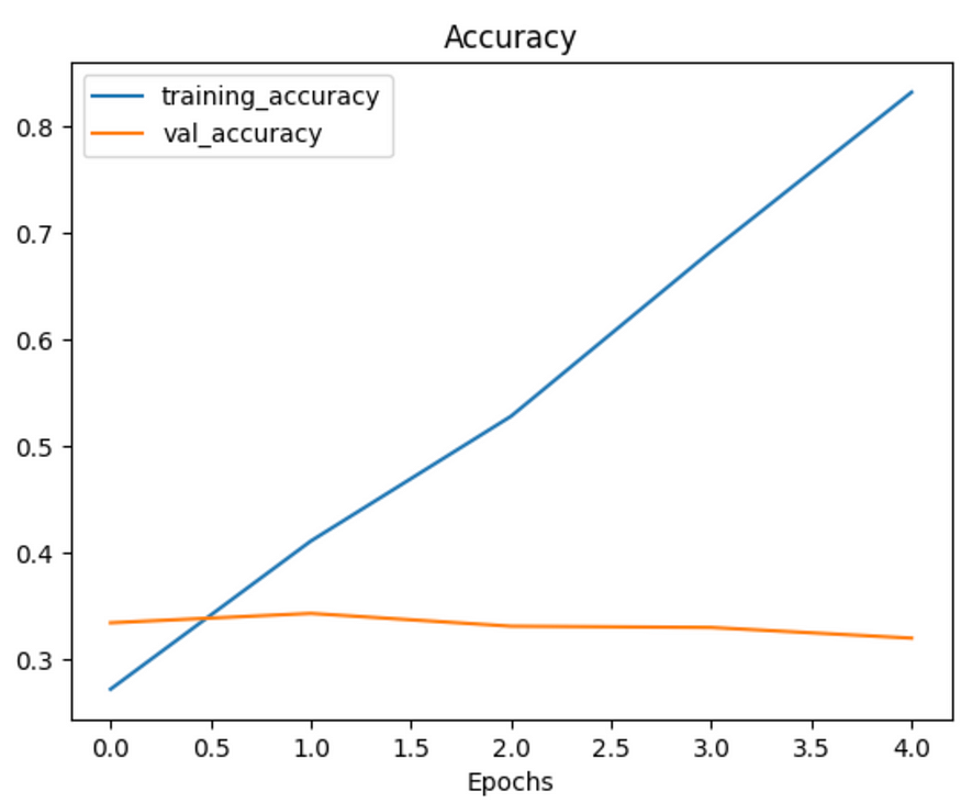
[6.493995189666748, 0.2556000053882599]# Check out the model's loss curves on the 10 classes of data (note: this function comes from above in the notebook)
plot_loss_curves(history_9)

he significant gap between the training and validation loss curves indeed indicates overfitting. This phenomenon occurs when a model learns the training data too well, including its noise and outliers, rather than generalizing from the patterns in the data. Here’s what this suggests about your model:
- High Training Accuracy, Low Validation Accuracy: If the model performs exceptionally well on the training data but poorly on the validation (or test) data, it suggests that the model has essentially ‘memorized’ the training data. It’s not effectively learning to generalize to new, unseen data.
- Lack of Generalization: The essence of a good model is its ability to perform well on data it hasn’t seen before. Overfitting undermines this, making the model less useful in real-world applications where it encounters new data.
To address overfitting, you can consider several strategies:
- Data Augmentation: If you haven’t already, implement more data augmentation techniques. This can help the model learn more generalized features rather than memorizing the training data.
- Regularization: Techniques like dropout, L1/L2 regularization can be effective. They penalize the model for complexity, encouraging it to learn simpler patterns that are more likely to be general.
- Reduce Model Complexity: If your model is very deep or has too many parameters, simplifying it might help. Overly complex models can easily overfit to training data.
- Early Stopping: Implement early stopping in your training process. This stops training when the validation loss stops improving, preventing overfitting.
- More Data: If possible, adding more diverse training data can help the model learn more general patterns.
- Cross-Validation: Use cross-validation techniques to ensure that the model performs consistently across different subsets of the training data.
- Hyperparameter Tuning: Experiment with different learning rates, batch sizes, and other hyperparameters.
- Transfer Learning: Use a pre-trained model and fine-tune it on your dataset. Pre-trained models have already learned a wide range of features and are less likely to overfit on a specific dataset.
Addressing overfitting is a crucial step towards building a robust and generalizable machine learning model. Each of these strategies can contribute to a more balanced learning process, ensuring that your model performs well not just on the training data but also in real-world scenarios.
# Try a simplified model (removed two layers)
model_10 = Sequential([
  Conv2D(10, 3, activation='relu', input_shape=(224, 224, 3)),
  MaxPool2D(),
  Conv2D(10, 3, activation='relu'),
  MaxPool2D(),
  Flatten(),
  Dense(10, activation='softmax')
])

model_10.compile(loss='categorical_crossentropy',
                 optimizer=tf.keras.optimizers.Adam(),
                 metrics=['accuracy'])

history_10 = model_10.fit(train_data,
                          epochs=5,
                          steps_per_epoch=len(train_data),
                          validation_data=test_data,
                          validation_steps=len(test_data))


Epoch 1/5
235/235 [==============================] - 46s 194ms/step - loss: 2.0671 - accuracy: 0.2721 - val_loss: 1.9153 - val_accuracy: 0.3344
Epoch 2/5
235/235 [==============================] - 29s 121ms/step - loss: 1.7378 - accuracy: 0.4111 - val_loss: 1.8689 - val_accuracy: 0.3432
Epoch 3/5
235/235 [==============================] - 29s 121ms/step - loss: 1.4138 - accuracy: 0.5281 - val_loss: 1.9583 - val_accuracy: 0.3312
Epoch 4/5
235/235 [==============================] - 28s 118ms/step - loss: 1.0030 - accuracy: 0.6831 - val_loss: 2.0870 - val_accuracy: 0.3300
Epoch 5/5
235/235 [==============================] - 30s 126ms/step - loss: 0.5791 - accuracy: 0.8320 - val_loss: 2.4825 - val_accuracy: 0.3200
# Check out the loss curves of model_10
plot_loss_curves(history_10)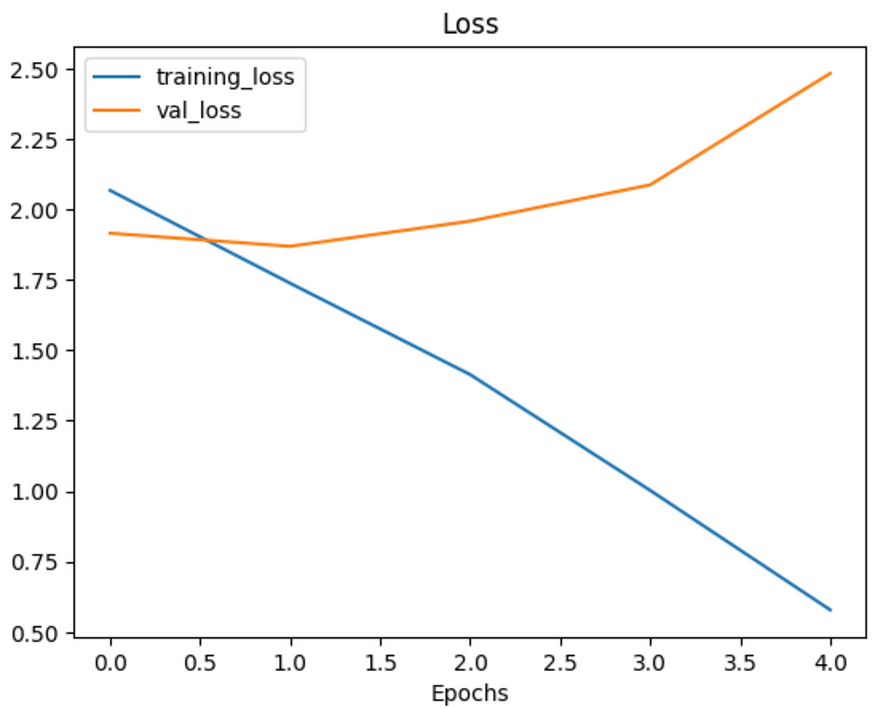
Even with a simplifed model, it looks like our model is still dramatically overfitting the training data.Data augmentation?
Data augmentation makes it harder for the model to learn on the training data and in turn, hopefully making the patterns it learns more generalizable to unseen data.
To create augmented data, we’ll recreate a new ImageDataGenerator instance, this time adding some parameters such as rotation_range and horizontal_flip to manipulate our images.
# Create augmented data generator instance
train_datagen_augmented = ImageDataGenerator(rescale=1/255.,
                                             rotation_range=20, # note: this is an int not a float
                                             width_shift_range=0.2,
                                             height_shift_range=0.2,
                                             zoom_range=0.2,
                                             horizontal_flip=True)

train_data_augmented = train_datagen_augmented.flow_from_directory(train_dir,
                                                                  target_size=(224, 224),
                                                                  batch_size=32,
                                                                  class_mode='categorical')
#Found 7500 images belonging to 10 classes.
Now we’ve got augmented data, let’s see how it works with the same model as before (model_10). Rather than rewrite the model from scratch, we can clone it using a handy function in TensorFlow called clone_model which can take an existing model and rebuild it in the same format. The cloned version will not include any of the weights (patterns) the original model has learned. So when we train it, it’ll be like training a model from scratch.
Note: One of the key practices in deep learning and machine learning in general is to be a serial experimenter. That’s what we’re doing here. Trying something, seeing if it works, then trying something else. A good experiment setup also keeps track of the things you change, for example, that’s why we’re using the same model as before but with different data. The model stays the same but the data changes, this will let us know if augmented training data has any influence over performance.
# Clone the model (use the same architecture)
model_11 = tf.keras.models.clone_model(model_10)

# Compile the cloned model (same setup as used for model_10)
model_11.compile(loss="categorical_crossentropy",
              optimizer=tf.keras.optimizers.Adam(),
              metrics=["accuracy"])

# Fit the model
history_11 = model_11.fit(train_data_augmented, # use augmented data
                          epochs=5,
                          steps_per_epoch=len(train_data_augmented),
                          validation_data=test_data,
                          validation_steps=len(test_data))

Epoch 1/5
235/235 [==============================] - 124s 517ms/step - loss: 2.1928 - accuracy: 0.1987 - val_loss: 2.0018 - val_accuracy: 0.3144
Epoch 2/5
235/235 [==============================] - 112s 474ms/step - loss: 2.0357 - accuracy: 0.2811 - val_loss: 1.8663 - val_accuracy: 0.3560
Epoch 3/5
235/235 [==============================] - 112s 478ms/step - loss: 2.0031 - accuracy: 0.3016 - val_loss: 1.8480 - val_accuracy: 0.3516
Epoch 4/5
235/235 [==============================] - 115s 489ms/step - loss: 1.9785 - accuracy: 0.3153 - val_loss: 1.7982 - val_accuracy: 0.3912
Epoch 5/5
235/235 [==============================] - 110s 467ms/step - loss: 1.9425 - accuracy: 0.3291 - val_loss: 1.7826 - val_accuracy: 0.3948
Each epoch takes longer than the previous model. This is because our data is being augmented on the fly on the CPU as it gets loaded onto the GPU, in turn, increasing the amount of time between each epoch.
# Check out our model's performance with augmented data
plot_loss_curves(history_11)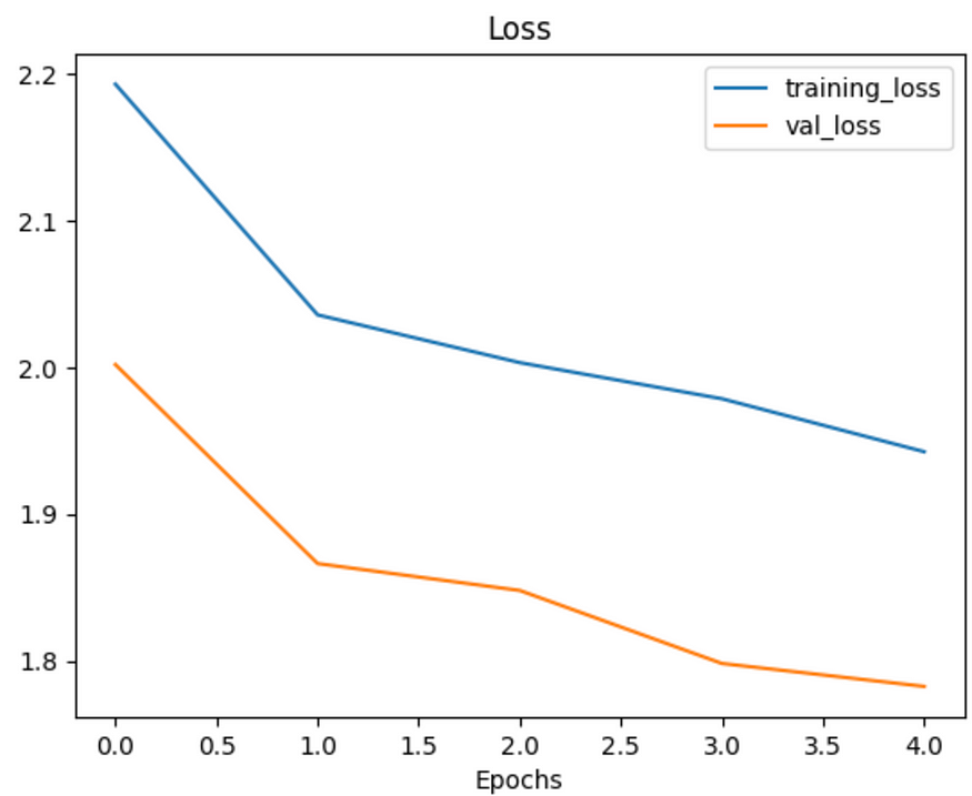

That’s looking much better, the loss curves are much closer to eachother. Although our model didn’t perform as well on the augmented training set, it performed much better on the validation dataset. It even looks like if we kept it training for longer (more epochs) the evaluation metrics might continue to improve.
Repeating until satisfied!
We could keep going here. Restructuring our model’s architecture, adding more layers, trying it out, adjusting the learning rate, trying it out, trying different methods of data augmentation, training for longer. But as you could image, this could take a fairly long time.
Good thing there’s still one trick we haven’t tried yet and that’s transfer learning. However, we’ll save that for the next notebook where you’ll see how rather than design our own models from scratch we leverage the patterns another model has learned for our own task.
In the meantime, let’s make a prediction with our trained multi-class model.
# What classes has our model been trained on?
class_names
#array(['chicken_curry', 'chicken_wings', 'fried_rice', 'grilled_salmon',
       'hamburger', 'ice_cream', 'pizza', 'ramen', 'steak', 'sushi'],
      dtype='<U14')
# -q is for "quiet"
!wget -q https://raw.githubusercontent.com/mrdbourke/tensorflow-deep-learning/main/images/03-pizza-dad.jpeg
!wget -q https://raw.githubusercontent.com/mrdbourke/tensorflow-deep-learning/main/images/03-steak.jpeg
!wget -q https://raw.githubusercontent.com/mrdbourke/tensorflow-deep-learning/main/images/03-hamburger.jpeg
!wget -q https://raw.githubusercontent.com/mrdbourke/tensorflow-deep-learning/main/images/03-sushi.jpeg
# Make a prediction using model_11
pred_and_plot(model=model_11,
filename="03-steak.jpeg",
class_names=class_names)
pred_and_plot(model_11, "03-sushi.jpeg", class_names)
# Load in and preprocess our custom image
img = load_and_prep_image("03-steak.jpeg")

# Make a prediction
pred = model_11.predict(tf.expand_dims(img, axis=0))

# Match the prediction class to the highest prediction probability
pred_class = class_names[pred.argmax()]
plt.imshow(img)
plt.title(pred_class)
plt.axis(False);
Much better! There must be something up with our pred_and_plot function. The pred_and_plot function was designed to be used with binary classification models where as our current model is a multi-class classification model.
The main difference lies in the output of the predict function.
# Adjust function to work with multi-class
def pred_and_plot(model, filename, class_names):
  """
  Imports an image located at filename, makes a prediction on it with
  a trained model and plots the image with the predicted class as the title.
  """
  # Import the target image and preprocess it
  img = load_and_prep_image(filename)

  # Make a prediction
  pred = model.predict(tf.expand_dims(img, axis=0))

  # Get the predicted class
  if len(pred[0]) > 1: # check for multi-class
    pred_class = class_names[pred.argmax()] # if more than one output, take the max
  else:
    pred_class = class_names[int(tf.round(pred)[0][0])] # if only one output, round

  # Plot the image and predicted class
  plt.imshow(img)
  plt.title(f"Prediction: {pred_class}")
  plt.axis(False);


pred_and_plot(model_11, "03-steak.jpeg", class_names)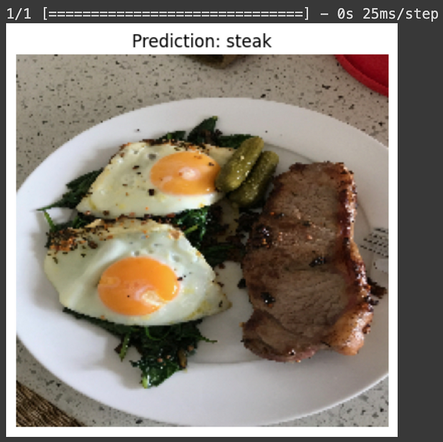
pred_and_plot(model_11, "03-sushi.jpeg", class_names)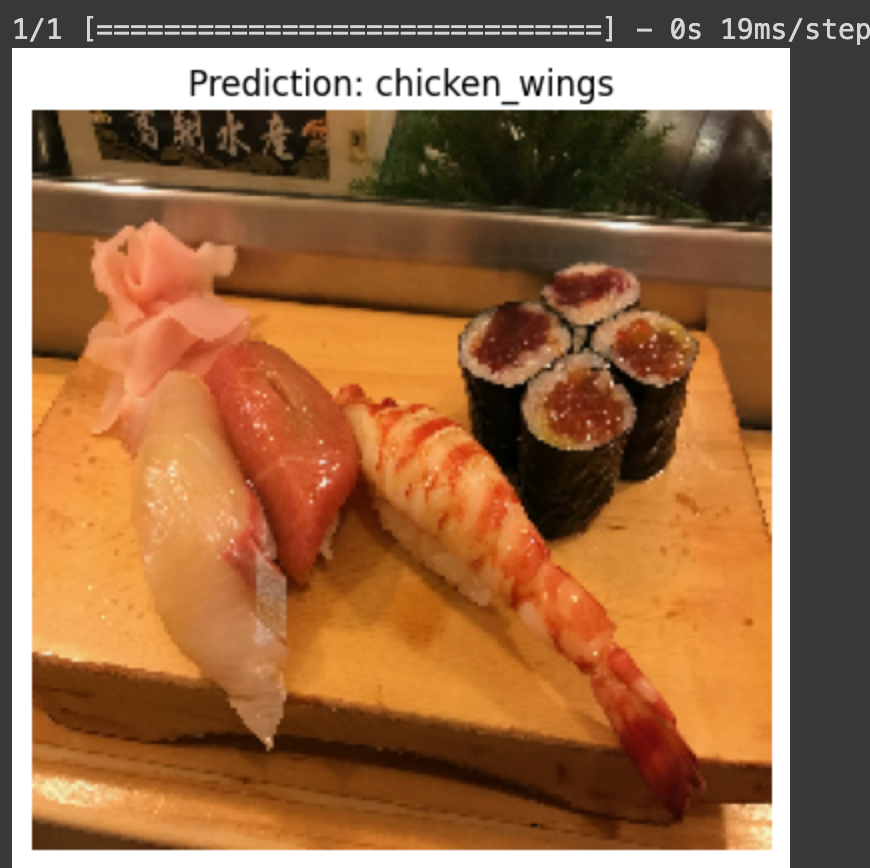
pred_and_plot(model_11, "03-hamburger.jpeg", class_names)
Our model’s predictions aren’t very good, this is because it’s only performing at ~35% accuracy on the test dataset. We’ll see how to improve this later on.
To conclude, our journey through the realms of CNNs and computer vision reveals a dynamic interplay of technology and practicality, where theoretical concepts transform into real-world applications. We have seen how CNNs, through their unique architecture and learning capabilities, adeptly handle complex visual data, paving the way for breakthroughs in various sectors.
The versatility and efficiency of CNNs in image recognition, object detection, and beyond signify a significant leap in how machines understand and interact with their visual environment. However, challenges such as overfitting and the need for extensive data highlight areas for future improvement and research. As we continue to advance in the field of AI and machine learning, CNNs stand as a testament to the profound impact of these technologies in shaping our visual and digital experiences.
If you would like to see more content related to my journey in data science, you can follow me on the following platforms.
linkedin.com/in/ali-kaan-erden-3725b719b
github.com/kaanerdenn
'Python' 카테고리의 다른 글
| [Errno 13] Permission denied: '/dev/ttyUSB0' (0) | 2024.05.02 |
|---|---|
| [Python] How to Run 70B LLMs on a Single 4GB GPU (0) | 2024.04.25 |
| [Python]Python GUI PyQt UI 생성 및 연결(Python GUI) (0) | 2024.04.24 |
| ESP32 cam Person Detection (0) | 2024.04.19 |
| Raspberry Pi NTP Server (0) | 2024.04.16 |


댓글