https://medium.com/@keur.plkar/audio-data-augmentation-in-python-a91600613e47
Audio Data Augmentation in python
In this post, I am going to show you how we can build a method for generating more samples in our dataset using data augmentation for…
medium.com
In this post, I am going to show you how we can build a method for generating more samples in our dataset using data augmentation for audio files.
Let’s get started
Data augmentation is a method for generating synthetic data i.e. creating new samples by tweaking small factors in the original samples. By altering these small factors we can get large amount of data for a single sample. This not only helps us to increase the size of our dataset but also gives multiple variations of single sample which helps our model to avoid overfitting and become more generalized.
We are going to use free-spoken-digit-dataset dataset. It is a free audio dataset of spoken digits. Think of it as MNIST for audio. It consists of 2000 recordings by 4 speakers (50 of each digit per speaker).
librosa, IPython.display.audio and matplotlib libraries are extensively used in this post. Before we continue It would be better to have a good background about these libraries.
Types of augmentation
Sound wave has following characteristics: Pitch, Loudness, Quality. We need to alter our samples around these characteristics in such a way that they only differ by small factor from original sample.
I found following alterations to a sound wave useful: Noise addition, Time shifting, Pitch shifting and Time stretching. We will see how these affects our original sample using spectrogram and play these altered audio files.
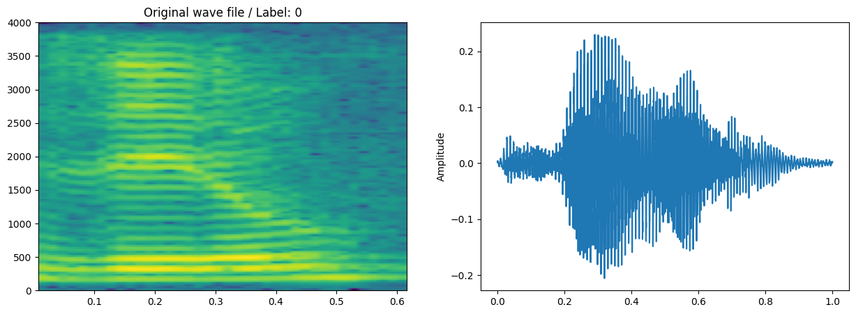
Visualizing original sample
We will use librosa to read the .wav file and matplotlib to generate spectrogram of wav file. Below is the code for visualization
Script for plotting spectrogram and amplitude graph
Visualizing original sample
import numpy as np
import matplotlib.pyplot as plt
import librosa

def plot_spec(data: np.array, sr: int, title: str, fpath: str) -> None:
    ''' Function for plotting spectrogram along with amplitude wave graph '''
    label = str(fpath).split('/')[-1].split('_')[0]
    fig, ax = plt.subplots(1, 2, figsize=(15, 5))
    ax[0].set_title(f'{title} / Label: {label}')
    ax[0].specgram(data, Fs=sr)  # Use 'sr' as the sampling frequency
    ax[1].set_ylabel('Amplitude')
    ax[1].plot(np.linspace(0, 1, len(data)), data)

# Set 'data_path' to a valid path before using it
data_path = "E:/vscode_workspace/free-spoken-digit-dataset/"

# Reading the wav file
#file_path = data_path.ls()[3]  # Make sure 'data_path' contains your file paths
file_path = os.listdir(data_path)[3]
print(file_path)
wav, sr = librosa.load(data_path+file_path, sr=None)

# Plotting the spectrogram and wave graph
plot_spec(wav, sr, 'Original wave file', file_path)

Original wave
Noise Addition
This process involves addition of noise i.e. white noise to the sample. White noises are random samples distributed at regular intervals with mean of 0 and standard deviation of 1.
For achieving this we will be using numpy’s normal method generate above distribution and add it to our original sample:
Script for adding white noise
'''
Noise addition using normal distribution with mean = 0 and std =1
Permissible noise factor value = x > 0.004
'''
import IPython.display as ipd

wav_n = wav + 0.009*np.random.normal(0,1,len(wav))
plot_spec(wav_n,sr,'Noise Added 0.005',file_path)
ipd.Audio(data=wav_n,rate=sr)
# librosa.output.write_wav('./noise_add.wav',wav_n,sr)
Time Shifting
Here we shift the wave by sample_rate/10 factor. This will move the wave to the right by given factor along time axis.
For achieving this I have used numpy’s roll function to generate time shifting.
Script adding time shift
#Shifting the sound wave
'''
Permissible factor values = sr/10
'''

wav_roll = np.roll(wav,int(sr/10))
plot_spec(data=wav_roll,sr=sr,title=f'Shfiting the wave by Times {sr/10}',fpath=file_path)
ipd.Audio(wav_roll,rate=sr)
# librosa.output.write_wav('./roll.wav',wav_roll,sr)
Time Stretching
The process of changing the speed/duration of sound without affecting the pitch of sound. This can be achieved using librosa’s time_stretch function.
Time_stretch function takes wave samples and a factor by which to stretch as inputs. I found that this factor should be 0.4 since it has a small difference with original sample.
Script for time stretching
#Time-stretching the wave
'''
Permissible factor values = 0 < x < 1.0
'''
factor = 0.4
wav_time_stch = librosa.effects.time_stretch(wav,rate=factor)
plot_spec(data=wav_time_stch,sr=sr,title=f'Stretching the time by {factor}',fpath=file_path)
ipd.Audio(wav_time_stch,rate=sr)
# librosa.output.write_wav('./time_stech.wav',wav_time_stch,sr)
Pitch Shifting
It is an implementation of pitch scaling used in musical instruments. It is a process of changing the pitch of sound without affect it’s speed.
Again we are going to use librosa’s pitch_shift function. It takes wave samples, sample rate and number of steps through which pitch must be shifted. I found that number of steps between -5 to 5 are much favorable as per our dataset.
Script for pitch shifting
#pitch shifting of wav
'''
Permissible factor values = -5 <= x <= 5
'''
wav_pitch_sf = librosa.effects.pitch_shift(wav,sr = sr,n_steps=-5)
plot_spec(data=wav_pitch_sf,sr=sr,title=f'Pitch shifting by {-5} steps',fpath=file_path)
ipd.Audio(wav_pitch_sf,rate=sr)
# librosa.output.write_wav('./pitch_shift.wav',wav_pitch_sf,sr)
You can find the complete jupyter notebook for audio data augmentation here
Audio Data Augmentation Visualization - librosa intgration - PART 2.ipynb
Audio Data Augmentation Visualization - librosa intgration - PART 2.ipynb - audio-data-augmentation-visualization-librosa-intgration-part-2.ipynb
gist.github.com
Congratulations you have successfully performed data augmentation on audio dataset.
'Python' 카테고리의 다른 글
| mqtt 참고사이트 (0) | 2024.03.19 |
|---|---|
| Object Distance & Direction Detection for Blind and Low Vision People (0) | 2024.01.26 |
| Data Augmentation in Python: Everything You Need to Know (0) | 2023.11.02 |
| [python]pyQt5 GUI Designer (0) | 2023.09.15 |
| [Python]Seaborn-Data (0) | 2023.09.05 |


댓글